I. Utility of Soil Resistivity Measurement
Soil electrical resistivity represents a key factor in the design of appropriate earthing systems because of its direct proportionality with the earthing resistance. This is also true when considering simple electrical design, dedicated low-resistance grounding systems, or more complex issues involved in the earth potential rise (EPR) studies. Appropriate soil surveys and models are the basis of all earthing designs and they are accomplished from an accurate soil resistivity testing.
II. Soil Resistivity Measurement Techniques
Soil electrical resistivity measurement might be carried out using different methods such as geological maps, seismic testing and ground penetrating radar. In these methods, the soil resistivity estimation is mainly based either on (i) electrodes spacing, or (ii) satellite imaging techniques [1].
Laboratory tests can be also performed on small soil samples for the resistivity measurement.
A. Satellite Imaging Based-Technique
From satellite or airborne sensors, measurement is carried out by detecting specific chemical and material bonds to estimate the soil electrical resistivity. In this remote sensing, information transfer is accomplished using electromagnetic radiation (EMR). According to the EMR source, sensing is classified into passive and active [2]. Passive sensing (left side of Fig. 1) is based on naturally occurring signals that can be received (i.e., radiation emitted by an object or reflected by an object) while active remote sensing, as shown in the right side of Fig. 1, provides its own radiation.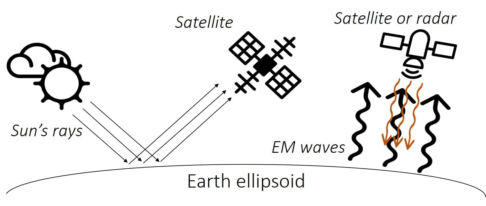
Actual materials detection mainly depends on the spectral coverage, spectrometer characterisation, material abundance and the strength of absorption features of that material in the wavelength region. Indeed, algorithms have been developed to exploit the spectral information obtained from the sensors as well as to better deal with the computational demands of these enormous data sets [2].
B. Electrodes Spacing Based-Technique
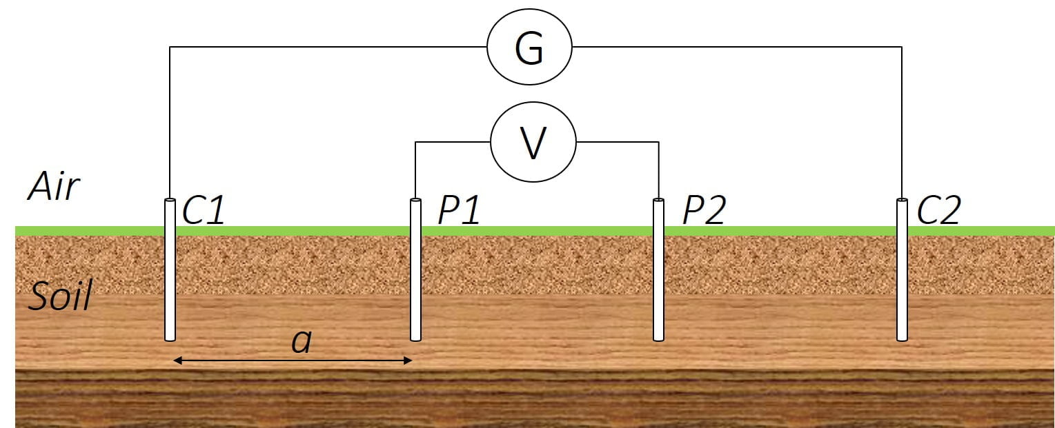
This technique is based on Ohm’s law, and the measurement principle usually consists of using four aligned electrodes. Several dispositions of the electrodes are feasible, and Wenner’s one is the most common electrode spacing technique. As shown in Fig. 2, a DC current “I” is injected between the two outer electrodes C1 and C2 (called current electrodes), and then the voltage “V” is measured between the two inner electrodes P1 and P2 (called potential electrodes) [3].The voltage current ratio (V/I) represents the resistance R of a volume of soil Henc e the soil apparent resistivity (p) is calculated as follows:
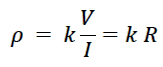
where, k is a geometric factor which depends on the arrangement of the testing electrodes.
In most cases, resistivity measurement records, usually expressed in Ω. 𝑚, should include temperature data and information on the moisture content of the soil at the time of measurement. Spacing distance is generally much greater than the driven depth [4]. Table I illustrates the mathematical expressions of the geometric factor ‘𝑘’ for the most common techniques of soil resistivity measurement.
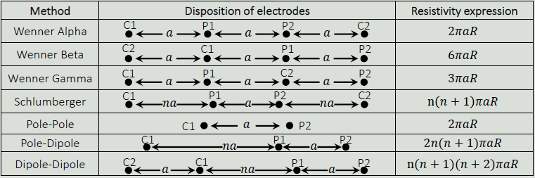
For a homogeneous soil, the measured resistivity will be approximately the same, whatever the combination adopted for the arrangement of the electrodes, which is not the case when the soil is not homogeneous as happens most often [5].
III. Practical guide to 2D and 3D surveys
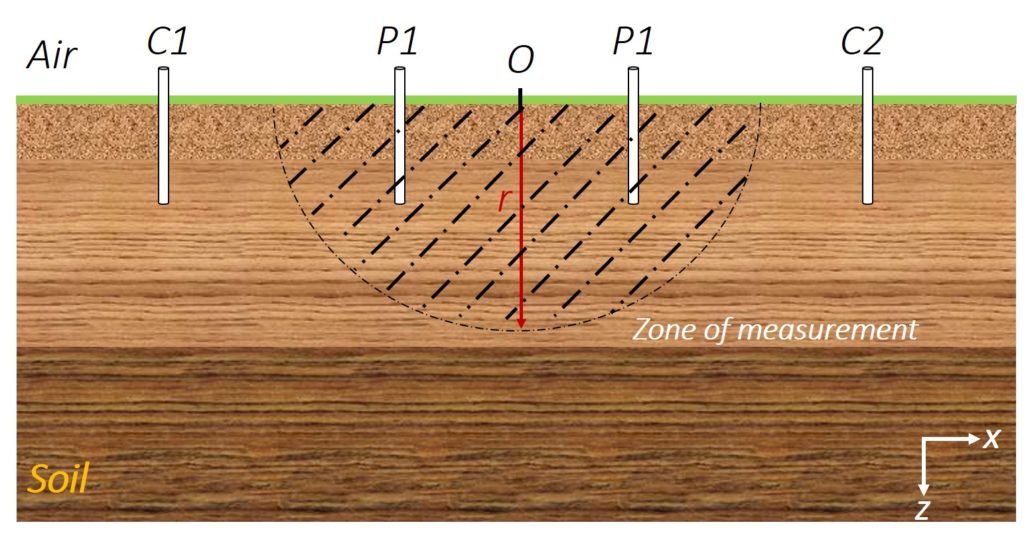
soil volume whose resistivity is measured is approximately a half-sphere whose center is in the middle of the station, in the point O, and whose diameter is equal to the separating distance (r=a). It will suffice to increase the value of a for the sounding to descend to a greater depth, which is called vertical sounding.Using Wenner system, one can gradually increase the spacing between the electrodes, keeping the same point as the station center.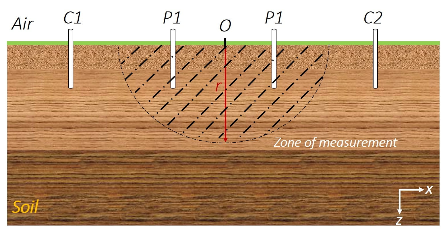
From a series of soundings, one will be able to estimate the resistivity of the layers that eventually make up the soil, and the approximate thickness of each one of them [4]. Indeed, horizontal surveys are much more common practice.
In 2D and 3D surveys, two main types of measurements might be used:
- HORIZONTAL SOUNDING: a series of measurements should be carried out by moving along a straight line; the line formed by the four electrodes being either parallel or perpendicular to the axis of this progression.
- VERTICAL SOUNDING: after having squared the ground, measurements are taken at each of the points of intersection of the lines forming the grid.
No heavy equipment is needed to perform this test. Nevertheless, the measurement requires some hard work and long time to determine a large-scale profile of soil resistivity.
IV. Soil Resistivity Modelling
2D profiles are the most practical and economic models that compromise between obtaining very accurate results and keeping the survey costs down.
A. 1D Soil Resistivity Modelling
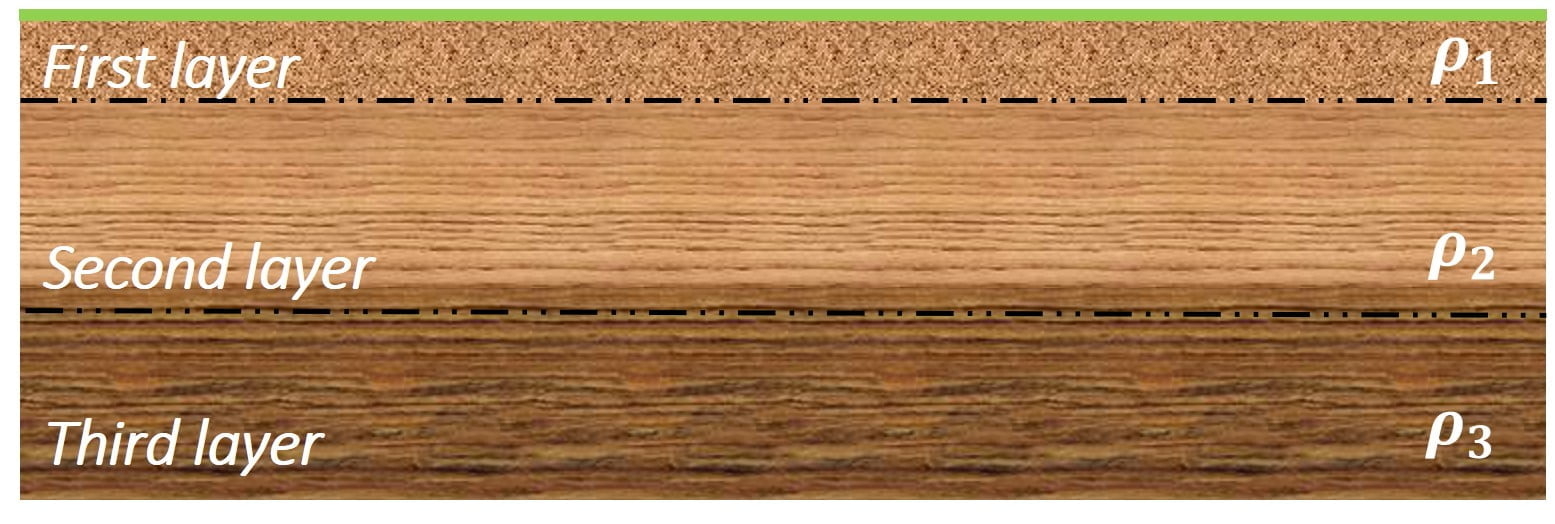
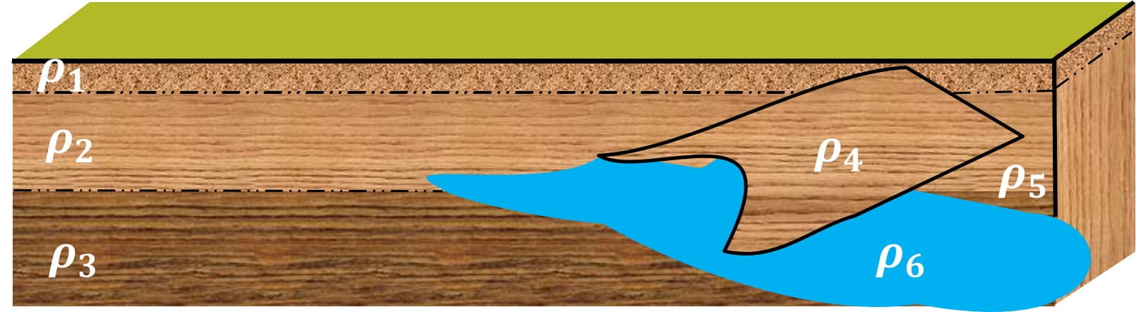
The 1D model assumes that the soil electrical resistivity varies in depth, depending on soil stratification as shown in Fig. 4.
According to IEEE Std 80 [3], two-layer structures are usually sufficient to lead to an acceptable design. Indeed, the soil stratification and number of layers can be determined after plotting the measured soil resistivity with respect to the distance between electrodes. Figure 5 shows example of the soil resistivity evolution versus spacing distance and their interpretation.
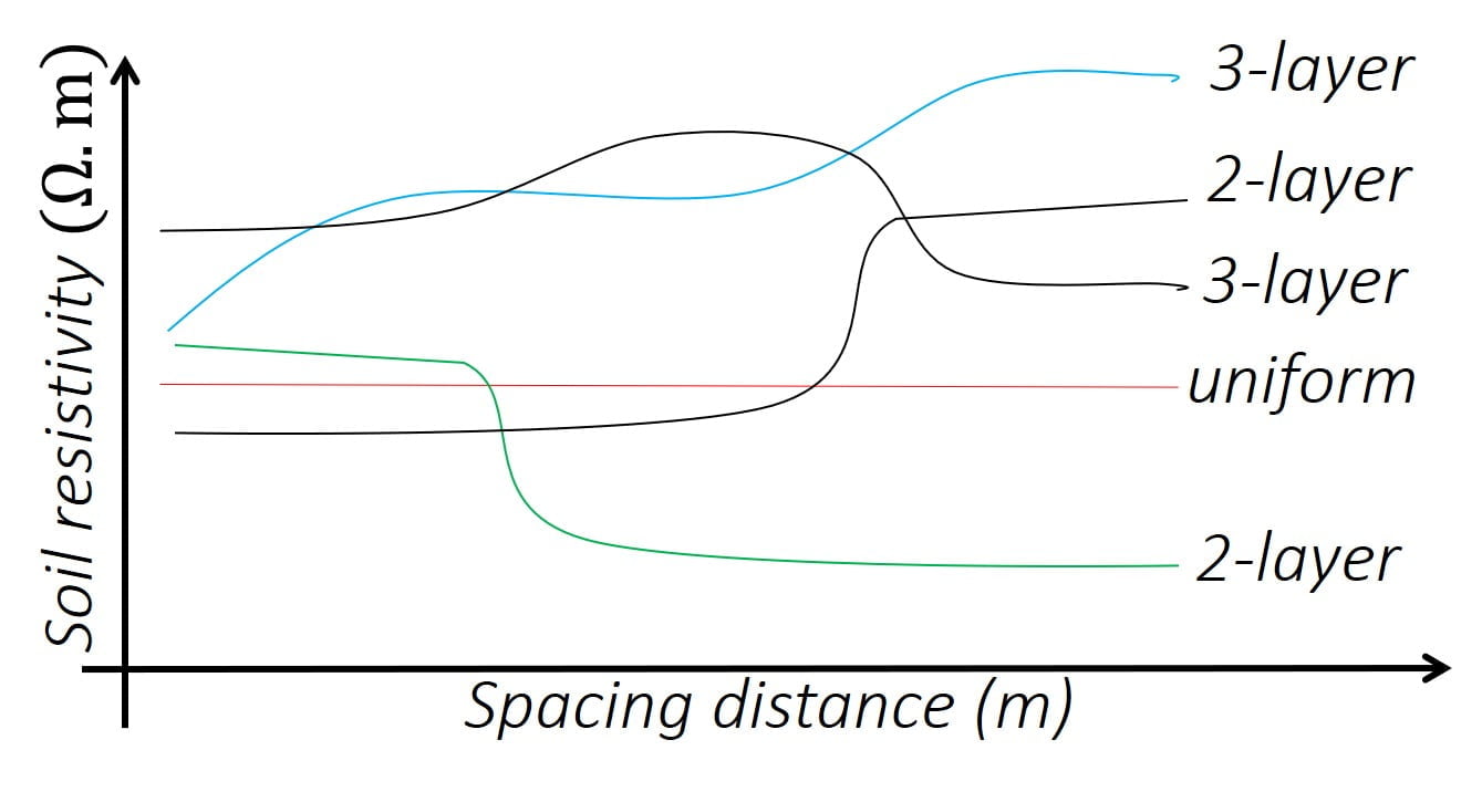
For a uniform soil, the apparent resistivity remains practically constant as function of the inter-electrode distance. Usually, one can use the uniform model when there is not a large difference between the resistivities of the different layers. In the case where the apparent resistivity increases (respectively decreases) as a function of the spacing distance, the results can be interpreted by two-layer soil model; an upper layer of low (respectively high) resistivity which covers a lower layer of high (respectively low) resistivity. It is worth noting that the same procedure should be respected for the more complex variation of soil resistivity, e.g., upper-curve shows that the soil can be represented by three-layer model.
B. 2D and 3D Soil Resistivity Modelling
In 1D Modelling, there is a limitation of the resistivity sounding method. This limitation consists in the neglection of the horizontal changes in the subsurface resistivity. For this purpose, a more accurate model of the subsurface is a 2D model. In this model, the resistivity changes in the vertical and horizontal directions as shown in Fig. 6.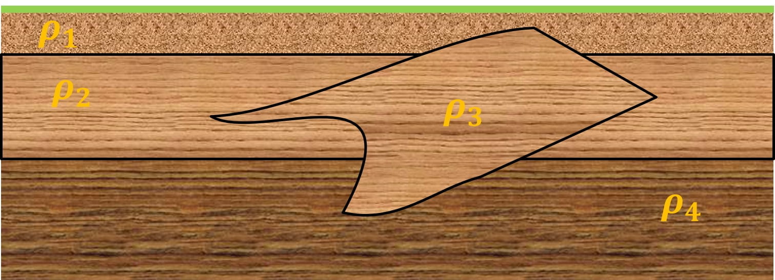
Series of measurements should be established using four-pin method. In each measurement, the distance between electrodes is changed for vertical soundings, while the position is changed for horizontal soundings. 3D modelling is clearly similar to the 2D modelling procedure.
In 3D model, a successive 2D models should be produced in parallel where its combination form the 3D model.
Build a 1D Soil Resistivity Model
Uniform soil models is widely performed to estimate the step and contact voltages. The approximate uniform soil resistivity can be considered as the arithmetic mean of the measured apparent resistivity data as follows [1]:
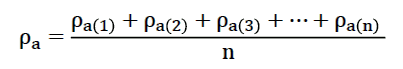
where, ρa (1) , ρa (2) , …, ρa (n) are the n measured resistivity at different spacings or depths.
A two-layer 1D soil resistivity model is characterised by three parameters, namely: the two resistivities of the upper and lower layers as well as the thickness of the upper layer. This soil model can be approximated by using different graphical methods described by Blattner-Dawalibi, Endrenyi, Sunde and others [1].
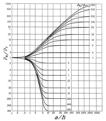
In Sunde’s method, the graph (based on the Wenner four-pin test data) shown in Fig. 8 is used to approximate a two-layer soil model.
- Plot a graph of apparent resistivity 𝜌𝑎 on y-axis versus pin spacing on x-axis.
- Estimate 𝜌1 and 𝜌2 from the graph plotted in a) where 𝜌𝑎 corresponding to a smaller spacing is 𝜌1 and for a larger spacing is 𝜌2. Extend the apparent resistivity graph at both ends to obtain these extreme resistivity values if the field data are insufficient.
- Determine 𝜌2/𝜌1 and select a curve on the Sunde’s graph, which matches closely, or interpolate and draw a new curve on the graph.
- Select the value on the y-axis of 𝜌𝑎/𝜌1 within the sloped region of the appropriate 𝜌2/𝜌1 curve of Sunde’s graph.
- Read the corresponding value of 𝑎/ℎ on the x-axis.
- Compute 𝜌𝑎 by multiplying the selected value by 𝜌1.
- Read the corresponding probe spacing from the apparent resistivity graph plotted in a). h) Compute h, the depth of the upper level, using the appropriate probe separation, a.
CDEGS is one of the few available software that can be used to compute the soil resistivity structure using the field test results. Multi-layer can be obtained as per the user specification.
Build a 2D Soil Resistivity Model
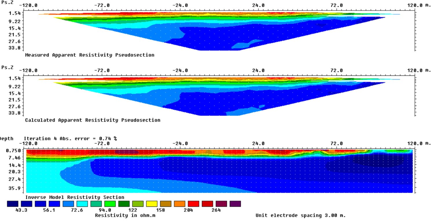
Typical 1D resistivity sounding surveys involve about 10 to 20 readings, while 2D imaging surveys involve approximately about 100 to 1000 measurements. In comparison, 3D surveys usually involve several thousand measurements [5]. Based on the measured apparent resistivity , 2D soil resistivity model can be produced in few seconds using RES2DINV.
RES2DINV is a computer program that use the smoothness-constrained Gauss-Newton least-squares inversion technique to produce a 2D model of the subsurface from electrical imaging surveys using the ABEM/Lund system. It supports the Wenner, Schlumberger, pole-pole, pole-dipole, dipole-dipole, multiple gradient and non-conventional arrays. Fig. 9 illustrates an example of the electrical image, of Cardiff University testing field, using RES2DINV.
References
[1] A. Sarris et al. (2018), An Introduction to Geophysical and Geochemical Methods in Digital Geoarchaeology. Digital Geoarchaeology, Springer.
[2] V. L. Mulder et al., “The use of remote sensing in soil and terrain Mapping — A review”, Geoderma, vol. 162, no. 1–2, pp. 1-19, Apr. 2011.
[3] IEEE Std 80-2013, IEEE Guide for Safety in AC Substation Grounding
[4] IEEE Std 81 Guide for measuring earth resistivity, ground impedance, and earth surface potentials of a ground system.
[5] M. H. Loke (2001), Electrical Imaging Surveys for Environmental and Engineering Studies. A Practical Guide to 2-D and 3-D Surveys.